The Sensitivity Matrix in Electrical Tomography

One-sentence definition

The sensitivity matrix (also called the Jacobian matrix) describes how much the measured capacitance / conductance / voltage between electrodes changes when the electrical constant (conductivity σ, permittivity ε or permeability μ) of a small region within the sensor’s field of view is slightly perturbed.

Mathematically it relates the “internal medium distribution” to the “boundary measurements” through a linear approximation:

ΔZ = S · Δγ

where ΔZ is the M-dimensional measurement-change vector, Δγ is the N-dimensional medium-distribution-change vector, and S is the M×N sensitivity matrix.

Every electrical tomography system — ECT, ERT, EMT, EIT — must first compute this S before image reconstruction.

What problem it solves

Tomography is fundamentally an inverse problem: you can only place electrodes on the boundary of the object, yet you want to know the electrical property of every pixel inside. Computing the boundary measurement from the internal distribution is the forward problem (easy, physically unique); the reverse is not — the same set of boundary measurements may correspond to multiple internal distributions.

The role of the sensitivity matrix is to locally linearise this non-linear, ill-posed inverse problem:

• Forward simplification: a first-order Taylor expansion near the known background distribution gives ΔZ ≈ S · Δγ
• Solvable inverse: linear-algebra tools (LBP, Tikhonov, Landweber, SVD…) can then back-compute Δγ
• Sensor evaluation: the row / column structure of S tells you which measurements and which regions carry enough information and which are “blind spots”

Two computation methods

Method A: perturbation method (intuitive but slow)

Compute straight from the definition: divide the field of view into N pixels, apply a small perturbation Δγ_i to each pixel i individually, run one forward simulation, and record the change ΔZ of all M measurements — that fills in column i.

• Pro: the principle is direct and works for any complex geometry
• Con: requires N forward solves; a typical ECT field of view has N = 1000–3000, so a slightly complex sensor structure takes hours

Method B: field method / reciprocity method (the engineering mainstream)

Using the reciprocity theorem of electromagnetic fields, sensitivity is written directly as the dot product of two field sets integrated over the pixel volume:

• Conductivity sensitivity S_σ = −∫ E_A · E_B dV
• Permittivity sensitivity S_ε = −jω ∫ E_A · E_B dV
• Permeability sensitivity S_μ = jω ∫ μ H_A · H_B dV
• Velocity sensitivity (electromagnetic flow tomography) S_v = ∫ (v × B_A) · E_B dV

where E_A, H_A are the field distributions when the excitation electrode is energised, and E_B, H_B are the field distributions when the measurement electrode is reverse-energised. Only n forward solves (n = number of electrode pairs) are needed to assemble the whole M×N matrix — 1 to 2 orders of magnitude faster than the perturbation method.

This is why commercial ECT/ERT software almost universally uses the field method.

What a sensitivity distribution looks like

Plot one row of S (corresponding to one measurement of one electrode pair) as a heat map by pixel position and you get a “sensitivity distribution map”. The characteristics differ greatly between sensor structures:

Figure: normalised sensitivity distributions for seven typical capacitance-electrode structures. (a) double concave / (b) multi-pair concave / (c) double helical / (d) staggered concave / (e) multi-helical / (f) double semi-cylinder / (g) ring. From Z. Cui et al., IEEE Sensors J., 21(24), 2021, Fig. 5.

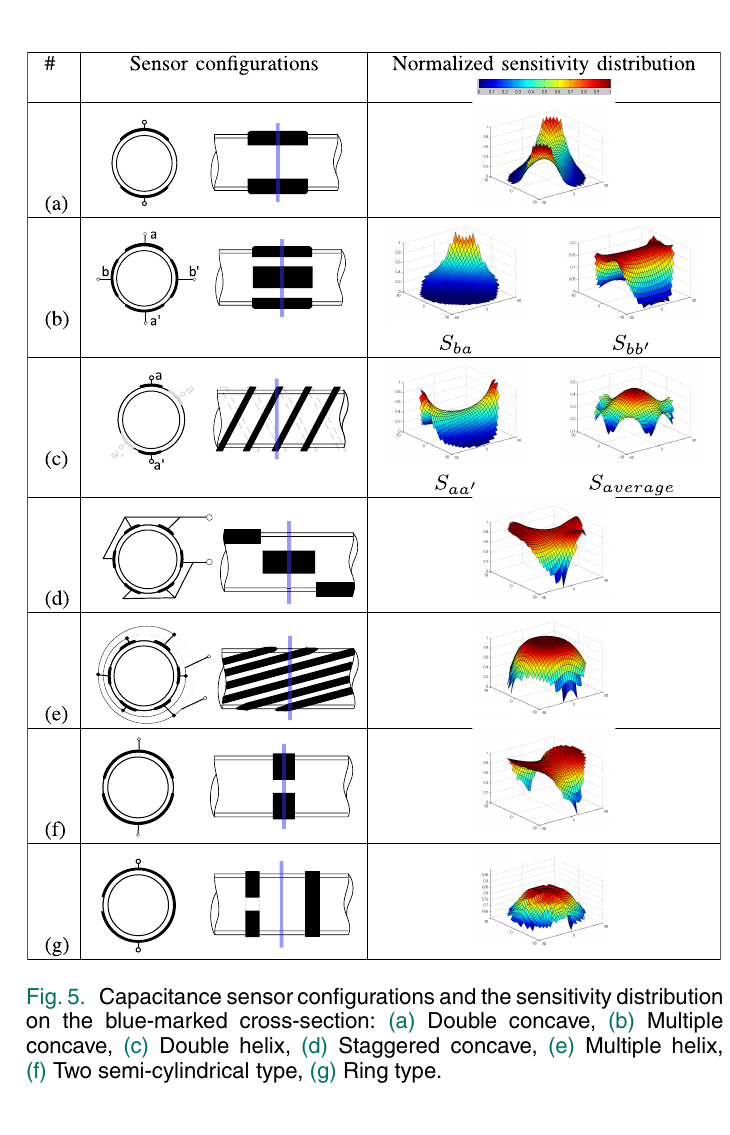
• Planar / coaxial electrode pair: essentially uniform across the cross-section — the ideal geometry for single-point fraction measurement
• Concave electrodes: a typical saddle shape — very high sensitivity near the electrodes, very low at the centre
• Helical electrodes: more uniform than concave because of the circumferential integration effect; suits stratified / annular flow
• Ring electrodes: high sensitivity near the wall; suits liquid-film-thickness measurement
• ECT / ERT arrays: each electrode pair has its own sensitivity “petal”; together they cover the cross-section, but information density at the centre is lower than at the wall

When designing an electrode structure, the goal is usually “make the sensitivity distribution as uniform as possible within the region of interest and as low as possible outside it” — this is commonly the objective function for electrode-geometry optimisation.

Soft field vs hard field: why electrical imaging has lower resolution than CT

X-ray CT is a hard field: rays travel in straight lines, each pixel’s contribution to the attenuation of each ray depends almost only on geometry, the sensitivity matrix is independent of the object’s contents, and the inverse problem is well-behaved.

Electrical tomography is a soft field: the electric / current field redistributes as the medium distribution changes, meaning the sensitivity matrix is actually a function of the medium distribution, S = S(γ). This has several direct consequences:

• Strictly speaking, ΔZ = S(γ) · Δγ is linear only in a small neighbourhood around γ
• A single computed S used for global reconstruction produces systematic error in regions far from the reference distribution
• To reduce that error, engineering practice often uses iterative reconstruction: each step first updates S with the current estimate of γ, then solves one more linear step
• This is the fundamental reason electrical tomography’s spatial resolution (~5% of pipe diameter) is far lower than CT’s (sub-millimetre)

Common uses in engineering

• Image reconstruction: linear algorithms (LBP, Tikhonov regularisation) use S^T or (S^T·S + λI)^-1·S^T directly; iterative algorithms (Landweber, conjugate gradient, neural networks) all use S as the forward model
• Sensor-design validation: before physically prototyping a new electrode structure, compute S by finite elements to check whether the sensitivity distribution matches expectations and whether there are “blind spots”
• Measurement selection: the M measurements are not equivalent — by analysing the correlation of the rows of S you can spot redundant measurements and design an under-sampling strategy to cut acquisition time
• Uncertainty assessment: the decay rate of S’s singular values reflects reconstruction stability; when the singular values span several orders of magnitude, stronger regularisation is needed
• Multi-modal fusion: stacking the sensitivity matrices of different modalities (ECT + ERT, ECT + ultrasound) enables joint reconstruction that fills in each other’s “blind spots”

Want to go deeper?

For the full derivation of the sensitivity matrix and its relationship with the five EMA models, see the review paper: Z. Cui, Q. Zhang, K. Gao, Z. Xia, H. Wang, “Electrical Impedance Sensors for Multi-Phase Flow Measurement: A Review”, IEEE Sensors Journal, Vol. 21, No. 24, Dec. 2021, pp. 27252–27267 (DOI: 10.1109/JSEN.2021.3124625). Section II gives the full derivation from Maxwell’s equations to the sensitivity formula and compares the sensitivity distributions of different electrode structures.

See also Z. Cui et al., “A review on image reconstruction algorithms for electrical capacitance/resistance tomography,” Sensor Review, Vol. 36, No. 4, 2016, pp. 429-445, which focuses on the use of the sensitivity matrix across the various reconstruction algorithms.

Next step

To build the overall framework first, read What Is Tomography; to understand how tomography infers fraction, read Measuring Phase Fraction with Tomography; for the selection stage see ERT vs ECT. If you are designing your own electrode structure, contact us with your field-of-view size and region of interest, and we can run a sensitivity analysis together.